Incidental Polysemanticity

Update: accepted to the Re-Align and BGPT workshops @ ICLR 2024!

One obstacle to interpreting neural networks is polysemanticity. This where a single neuron represents multiple features.

If there are more features than neurons, it might be "necessary" for the model to be polysemantic in order to represent everything. This is the notion of "superposition" from Elhage et al. (2022).

Of course, a clear solution would be to train a model large enough to have at least one neuron per feature. However, what we find in "What Causes Polysemanticity?" is that polysemanticity can happen "incidentally" in the training process, even if we have a large enough model.

Hypothesis

When we initialise a neural network, the weights are random. Some neurons will be more correlated with some features than other neurons, just by chance.

As training happens, the optimiser pushes the weights of those correlated neurons in the direction of the features, so that they can represent the features well. If there is pressure for sparsity, only one neuron will represent each feature.

Most likely, this is the neuron which was most correlated to the feature at initialisation. If it happened to be the most correlated neuron for multiple features, then it would end up representing multiple features.

In that case, we get polysemanticity "incidentally".

Experiments

To test this hypothesis, we consider the simplest possible setup: over-parameterised autoencoders similar to those in Elhage et al. (2022). That is:

y = ReLU (W W^{T} x)

where $x \in ℝ^{n}$ and $W \in ℝ^{n \times m}$ , with $m \geq n$ . These models were trained on the standard basis vectors $e_{i} \in ℝ^{n}$ . To induce sparsity, we take two separate approaches: introducing $ℓ_{1}$ regularisation for the model weights and adding noise after the hidden layer.

We find that:

$ℓ_{1}$ regularisation induces sparsity
Some types of noise can induce sparisty
The amount of incidental polysemanticity can be predicted
It is due to the weight initialisations

Sparsity from Regularisation

Result 1: $ℓ_{1}$ regularisation induces a winner-takes-all dynamic at a rate proportional to the regularisation parameter.

Loss with $ℓ_{1}$

Taking the $i$ th basis vector as the input, the output of the model is:

(ReLU (W_{1, :} \cdot W_{i, :}), \dots, ReLU (W_{n, :} \cdot W_{i, :}))

With $ℓ_{1}$ regularisation, our loss function becomes:

ℒ = \sum_{i} (ReLU (W_{i, :} \cdot W_{i, :}) - 1)^{2} + \sum_{i} \sum_{j \neq i} (ReLU (W_{i, :} \cdot W_{j, :}) - 0)^{2} + \sum_{i} λ ‖ W_{i, :} ‖_{1}

where $λ$ is the regularisation parameter.

Thus, gradient descent pushes us in the direction:

- \frac{\partial ℒ}{\partial W_{i, :}} = (4 ‖ W_{i, :} ‖_{2}^{2} - 1) W_{i, :} - 4 \sum_{j \neq i} ReLU (W_{i, :} \cdot W_{j, :}) W_{j, :} - λ sign (W_{i, :})

Forces for sparsity

We can split this into the three terms:

Feature benefitThis is why we can use tied weights $W^{T}$ and $W$ , since it should push the $i$ th column of $W_{enc}$ and the $i$ th row of $W_{dec}$ to have dot product of $1$ , even if initialised as untied weights.: pushes $W_{i, :}$ to be unit length
Interference: pushes $W_{i, :}$ to be orthogonal to other $W_{j, :}$
Regularisation: pushes non-zero $W_{i, :}$ to be sparse

The feature benefit and regularisation forces are in competition. Since the regularisation force has a constant value while the feature benefit force is proportional to the length of $W_{i, :}$ , the regularisation force will dominate for small $W_{i, :}$ and the feature benefit force will dominate for large $W_{i, :}$ .

Thus $W_{i, k}$ will be pushed to $0$ if it is below some threshold $θ$ . Leaving the derivations for the paper, we find the net effect on sparsity is proportional to how far the weight is from this threshold:

\frac{d | W_{i, k} |}{d t} = (1 - ‖ W_{i, :} ‖_{2}^{2}) (| W_{i, k} | - θ)

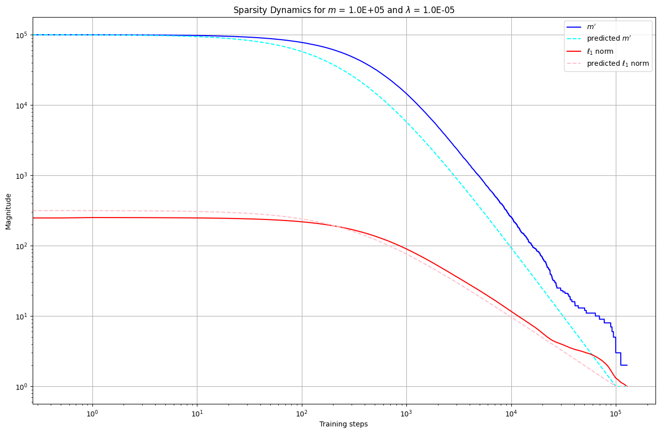
Speed of sparsification

In fact, we can quantify the speed at which sparsity is induced. Again, leaving the maths for the paper, it follows from above that the $ℓ_{1}$ norm at time $t$ is inversely proportional to $λ t$ :

‖ W_{i, :} (t) ‖_{1} = \frac{1}{Θ (\frac{1}{m} + λ t)}

Since $‖ W_{i, :} (t) ‖ \approx 1$ throughout training, the $m^{'}$ non-zero values at any particular point should have a magnitude of around $\frac{1}{\sqrt{m^{'}}}$ , and so $‖ W_{i, :} (t) ‖_{1} \approx m^{'} \frac{1}{\sqrt{m^{'}}} = \sqrt{m^{'}}$ . Thus the weights should go from $Θ (\sqrt{m})$ to $Θ (\frac{1}{λ t})$ as $t \geq \frac{1}{λ \sqrt{m}}$ and $Θ (1)$ as $t \geq \frac{1}{λ}$ . This is exactly what we see:

Sparsity from Noise

Result 2: noise drawn from a distribution with excess kurtosis induces sparsity.

Implicit regularisation

In practice, we don't get sparsity in neural networks because of $ℓ_{1}$ regularisation. A more realistic cause is via noise in the hidden layer, a la Bricken et al. (2023):

y = ReLU (W (W^{T} x + ξ))

for $ξ \in ℝ^{m}$ and $ξ ~ 𝒟$ . Having removed the regularisation term, the loss is rotationally symmetric with respect to the hidden layer (excluding the noise). That means there is no privileged basis, and no particular reason for features to be represented by a single neuron, as opposed to a linear combination of features.

However, if we take the noise into account, we find that one term in the loss is:

‖ W_{i, :} ‖_{4}^{4} (\frac{μ_{4}}{σ^{4}} - 3)

where $μ_{4}$ is the fourth moment of $𝒟$ , and $\frac{μ_{4}}{σ^{4}} - 3$ is the excess kurtosis.

Thus, when $𝒟$ has negative excess kurtosis, this component of the loss will push to increase $‖ W_{i, :} ‖_{4}$ . Due to the constraint that $‖ W_{i, :} ‖_{2} = 1$ from before, this incentivises $W_{i, j} = \pm 1$ for some $j$ and $W_{i, k} = 0$ for $k \neq j$ .

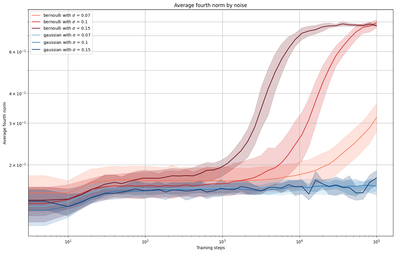
Bernoulli vs. Gaussian noise

Bernoulli noise of either $\pm σ$ has excess kurtosis of $- 2$ , while Gaussian noise has excess kurtosis of $0$ . Thus we would expect to see the former to induce sparsity (and a fourth norm of $1$ ), while the latter would not. As expected:

Counting Hypothesis

Result 3: the number of polysemantic neurons can be predicted by a simple combinatorial model.

Possible model solutions

Recall that the output of the autoencoder is:

(ReLU (W_{1, :} \cdot W_{i, :}), \dots, ReLU (W_{n, :} \cdot W_{i, :}))

That is, we would like $W_{i, :} \cdot W_{i, :} = 1$ and $W_{i, :} \cdot W_{j, :} \leq 0$ for $i \neq j$ .

One way to satisfy this is if $W_{i, :}$ equals the $i$ th standard basis vector $f_{i} \in ℝ^{m}$ . This is because $W W^{T}$ will just be the identity matrix, and so $ReLU (W W^{T} e_{i}) = e_{i}$ .

However, when $m > n$ , we have another solution. Take $m = 4$ and $n = 2$ , and consider the following weight matrix:

W = [\begin{matrix} 1 & 0 & 0 & 0 \\ - 1 & 0 & 0 & 0 \end{matrix}]

We see that $ReLU (W W^{T} e_{1}) = (1, 0)$ and $ReLU (W W^{T} e_{2}) = (0, 1)$ , which still satisfying the constraints. This is a polysemantic solution!

Interference force

Knowing that it is possible, we can now ask why it occurs. One force we haven't considered in detail is the interference force:

- \sum_{j \neq i} ReLU (W_{i, :} \cdot W_{j, :}) W_{j, :}

up to constants.

This is only non-zero if the angle between $W_{i, :}$ and $W_{j, :}$ is less than $\frac{π}{2}$ . Thus, we can simplify by only considering its effect in the direction of $W_{i, :}$ . It has magnitude:

(\sum_{j \neq i} ReLU (W_{i, :} \cdot W_{j, :}) W_{j, :}) \cdot W_{i, :} = \sum_{j \neq i} ReLU (W_{i, :} \cdot W_{j, :})^{2}

This means that the interference force should be weak at the start when $W_{i, :} \cdot W_{j, :}$ are mean zero, and only kick in $W_{i, :}$ and $W_{j, :}$ share some non-zero coordinate $k$ . If $W_{i, k}$ and $W_{j, k}$ have the same sign, the interference force will push at least one to zero. Thus, we would only expect that polysemanticity occurs when they have the opposite sign, since the ReLU will zero out the negative term and they will maintain their non-zero value.

Balls and bins

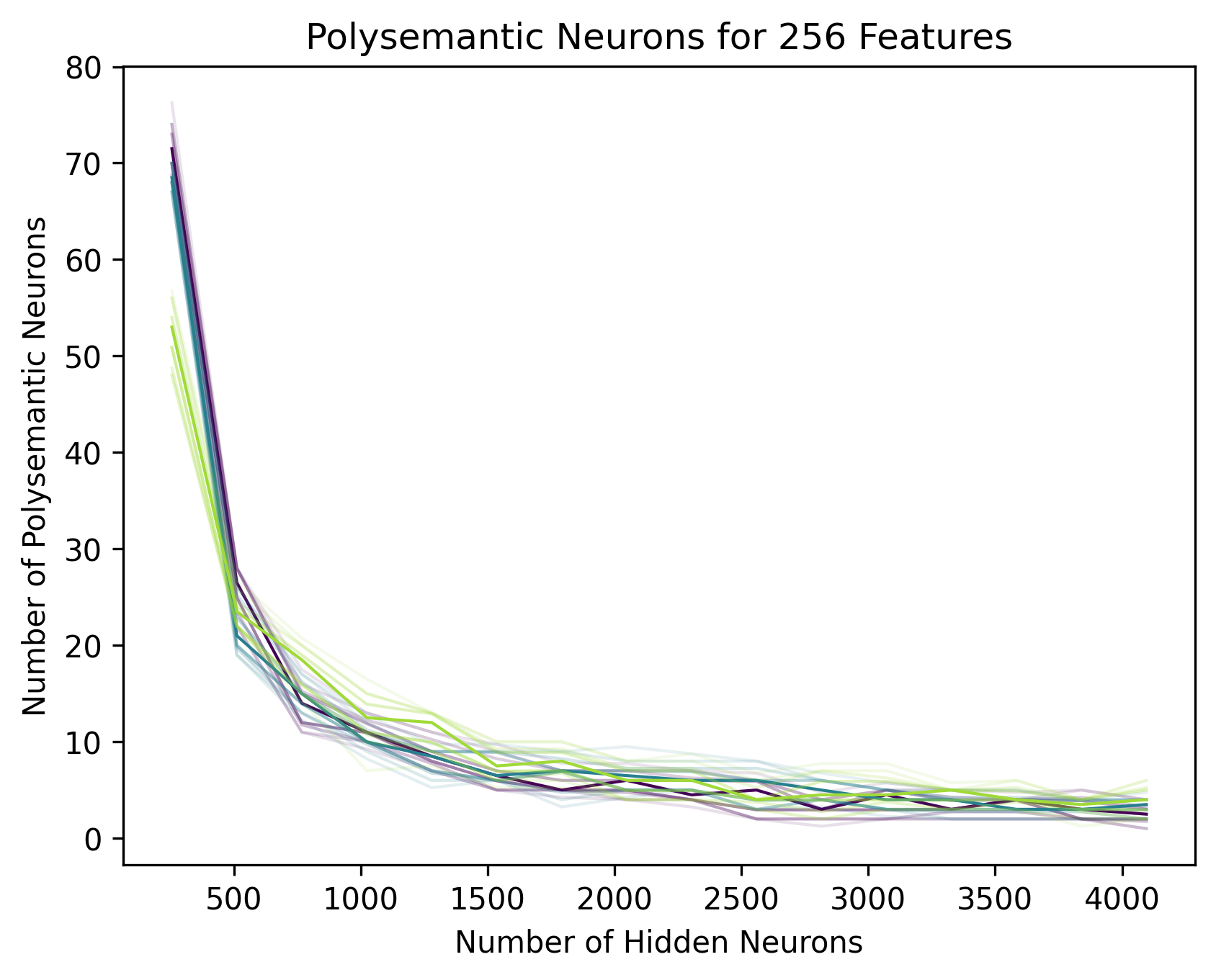
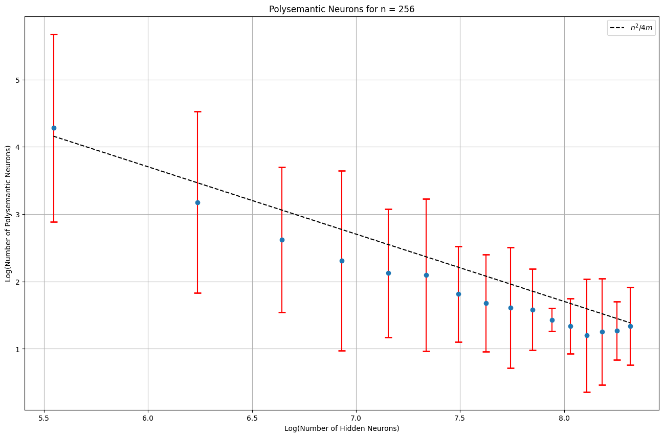
With $(\binom{n}{2})$ pairs of features, $\frac{1}{m}$ probability of the most significant neuron being the same for both and $\frac{1}{2}$ probability of them having the opposite sign, we would predict there to be $(\binom{n}{2}) \frac{1}{2 m} \approx \frac{n^{2}}{4 m}$ polysemantic neurons, which we find:

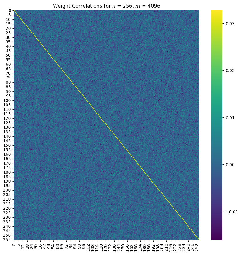
Initialisation Hypothesis

Result 4: polysemanticity occurs in $m > n$ models due to weight initialisations.

If initialisations were the cause of polysemanticity, the weights at the start of training should be correlated with the weights at the end. That is, the diagonals of $W W^{T}$ should be larger than the off-diagonals. As predicted:

Future Work

The incidental polysemanticity we have discussed in our work is qualitatively different from necessary polysemanticity, because it arises from the learning dynamics inducing a privileged basis. Furthermore, the fact that it occurs all the way up to $m = n^{2}$ suggests that making the model larger may not solve the problem.

We look forward to future work which investigates this phenomenon in more fleshed-out settings, and which attempts to nudge the learning dynamics to stop it from occurring.

If you want to play with different configurations of our models or reproduce our plots, check out the code repository!